Module `iceflow`

Brief summary

The iceflow module allows to determine the horizontal velocities \((u,v)\) of the ice. To do so, it solves higher-order ice-flow equations by minimizing an associated energy. This can be done in a traditional way, by computing the velocities each the time the glacier configuration changes, or, instead, by training a neural network that maps that configuration to the velocities. The parameters of the module are described here.

Transition to unified mode

The unified framework (method=unified) is the recommended approach going forward. It consolidates the legacy solver (method=solved) and emulator (method=emulated) into a single architecture where the computational strategy is selected via the mapping parameter. Legacy modes are still supported for backward compatibility, but new projects should use the unified mode; it offers new features (e.g., additional optimizers and stopping criteria) and greater flexibility (e.g., support for custom mappings).

The iceflow module is described in further detail in (The IGM developers, in prep.)¹.

State variables

Reads: thk, usurf, topg, arrhenius

Writes: U, V, ubar, vbar

Quick start-up guide

The iceflow module can be configured in different ways. All modes solve the same physical problem; the difference is how the solution is computed.

Legacy modes

Legacy stack — kept for backward compatibility only

The solved and emulated modes are kept for backward compatibility only and will be removed in a future version — prefer unified. On the legacy stack the basal friction is set with sliding.slidingco (MPa) — not sliding.tau_ref, which is unified-only — and sliding.u_ref must stay 1.0 (any other value is refused at startup). See the v3.1 → v3.2 migration guide.

Solved mode

Classical solve for the velocity field. Example configuration file:

iceflow:
  physics:
    sliding:
      slidingco: 0.0464       # Basal friction coefficient (legacy stack; MPa)
      u_ref: 1.0              # legacy (solved/emulated) stack requires u_ref = 1.0
    viscosity:
      arrhenius: 78.0         # Flow law coefficient (MPa^{-3} y^{-1})
  method: solved                # Classical solve
  solver:
    optimizer: adam             # Optimization algorithm
    step_size: 1.0              # Step size for optimizer
    nbitmax: 100                # Maximum number of iterations

Emulated mode

Training of a neural network that emulates the velocity field. Example configuration file:

iceflow:
  physics:
    sliding:
      slidingco: 0.0464       # Basal friction coefficient (legacy stack; MPa)
      u_ref: 1.0              # legacy (solved/emulated) stack requires u_ref = 1.0
    viscosity:
      arrhenius: 78.0         # Flow law coefficient (MPa^{-3} y^{-1})
  method: emulated              # Neural-network emulation
  emulator:
    pretrained: true            # Use pre-trained network
    lr: 2.0e-05                 # Learning rate
    retrain_freq: 10            # Retrain frequency (every 10 time steps)
    nbit: 1                     # Number of training iterations per time step

Unified mode

In the unified framework, the computational strategy is selected via the mapping parameter.

Identity mapping

Classical solve for the velocity field. Example configuration file:

iceflow:
  physics:
    sliding:
      tau_ref: 0.2154         # Basal shear stress (MPa, at default u_ref=100)
    viscosity:
      arrhenius: 78.0         # Flow law coefficient (MPa^{-3} y^{-1})
  method: unified               # Unified framework
  unified:
    mapping: identity           # Classical solve
    optimizer: lbfgs            # L-BFGS optimizer
    nbit: 100                   # Number of optimization iterations
    retrain_freq: 1             # Retrain frequency (solve at every iteration)

Network mapping

Training of a neural network that emulates the velocity field. Example configuration file:

iceflow:
  physics:
    sliding:
      tau_ref: 0.2154         # Basal shear stress (MPa, at default u_ref=100)
    viscosity:
      arrhenius: 78.0         # Flow law coefficient (MPa^{-3} y^{-1})
  method: unified               # Unified framework
  unified:
    mapping: network            # Neural-network emulation
    optimizer: adam             # Adam optimizer
    retrain_freq: 10            # Retrain frequency (every 10 time steps)
    nbit: 1                     # Number of training iterations per time step
    adam:
      lr: 2.0e-05               # Learning rate
    network:
      pretrained: true          # Use pre-trained network

Additional options

The unified framework allows additional options, for instance boundary conditions and multi-stage optimization:

iceflow:
  physics:
    sliding:
      tau_ref: 0.2154         # Basal shear stress (MPa, at default u_ref=100)
    viscosity:
      arrhenius: 78.0         # Flow law coefficient (MPa^{-3} y^{-1})
  method: unified               # Unified framework
  unified:
    mapping: network            # Neural-network emulation
    bcs: [frozen_bed]           # Boundary conditions
    optimizer: sequential       # Multi-stage optimization
    sequential:
      stages:
        - optimizer: adam       # Stage 1: Adam optimizer
          nbit: 10000           # 10000 iterations
        - optimizer: lbfgs      # Stage 2: L-BFGS optimizer
          nbit: 1000            # 1000 iterations

Physical model

Ice flow is governed by momentum balance and mass conservation. For glaciers and ice sheets with shallow geometry (horizontal extent ≫ thickness) and cryostatic vertical stresses, the three-dimensional Stokes equations reduce to the Blatter-Pattyn higher-order model (Herterich, 1987; Blatter, 1995; Pattyn, 2003)² ³ ⁴, a system of coupled, nonlinear, elliptic PDEs for the horizontal velocity field \(\mathbf{u}=(u,v)\).

Minimization formulation

Rather than solving these PDEs directly, IGM adopts an energy minimization approach (Jouvet & Rappaz, 2011; Jouvet, 2016)⁵ ⁶. The main advantage is that various optimizers can be applied to minimize this energy; in particular, both classical and neural-network approaches (Jouvet & Cordonnier, 2023)⁷.

The velocity field \(\mathbf{u}\) that satisfies the momentum balance is the one that minimizes the mechanical energy functional:

\[ \mathcal{J}(\mathbf{u}) = {\int_{\Omega} \frac{2\,A^{-1/n}}{1+1/n} \vert \mathbf{D}(\mathbf{u}) \vert^{1+1/n}\,\mathrm{d}\Omega} + {\int_{\Gamma_\mathrm{b}} \frac{c \vert\mathbf{u}_\mathrm{b}\vert^{1+1/m}}{1+1/m}\,\mathrm{d}\Gamma} - {\int_{\Omega} \rho_\mathrm{i} g \,\nabla s \cdot \mathbf{u}\,\mathrm{d}\Omega} - {\int_{\Gamma_\mathrm{cf}} \left[\rho_\mathrm{i} g (s-z) - p_\mathrm{w}\right] \mathbf{u}\cdot\mathbf{n}\,\mathrm{d}\Gamma}, \]

where \(\Omega\) is the three-dimensional ice domain, \(\Gamma_\mathrm{b}\) is the basal boundary, \(\Gamma_\mathrm{cf}\) is the calving front (absent for land-terminating glaciers), and \(s\) is the upper surface elevation. The four terms correspond to different physical processes:

The first term represents viscous dissipation. Here, \(\mathbf{D}(\mathbf{u}) = (\nabla \mathbf{u} + \nabla \mathbf{u}^\top)/2\) is the strain-rate tensor, \(A\) is the Arrhenius factor, and \(n\) is the flow law exponent.
The second term represents basal friction dissipation, here parametrized with a Weertman law. Here, \(c\) is the friction coefficient, \(\mathbf{u}_\mathrm{b}\) is the basal velocity, and \(m\) is the power-law exponent.
The third term represents gravitational power, which is the driving force. Here, \(\rho_\mathrm{i}\) is ice density and \(g\) is gravitational acceleration.
The fourth term accounts for the calving-front energy in marine-terminating glaciers, where \(p_\mathrm{w}\) is the hydrostatic water pressure and \(\mathbf{n}\) is the outward horizontal unit normal to \(\Gamma_\mathrm{cf}\).

The ice velocity is found by minimizing this functional:

\[ \mathbf{u} = \arg\min_{\mathbf{{ v }}} \mathcal{J}(\mathbf{v}; c, A, h, s), \]

where the functional depends on the evolving glacier state through the following variables:

basal friction coefficient \(c\);
Arrhenius factor \(A\);
ice thickness \(h\);
surface elevation \(s\).

Numerical set-up

To make the continuous energy minimization problem computationally tractable, we discretize the velocity field on a structured grid. This discretization transforms the infinite-dimensional optimization problem into a finite-dimensional one where the unknowns are velocity degrees of freedom, typically velocity values at discrete spatial locations.

Horizontal discretization

The horizontal domain is discretized on a uniform rectangular grid of size \(N_x \times N_y\) with constant cell spacing \(H =\Delta x = \Delta y\). Discrete variables such as friction coefficient \(c_H\), flow law coefficient \(A_H\), ice thickness \(h_H\), and surface elevation \(s_H\) are defined at grid cell corners. We use subscript \(H\) to denote these discrete quantities defined on the horizontal grid. These discrete fields are represented as 2D tensors: \(\mathbf{c}_H, \mathbf{A}_H, \mathbf{h}_H, \mathbf{s}_H \in \mathbb{R}^{N_y \times N_x}\). At a grid point \((x_i, y_j)\), the discrete values are denoted:

\[ (\mathbf{c}_H)_{j,i} = c(x_i, y_j), \quad (\mathbf{A}_H)_{j,i} = A(x_i, y_j), \quad (\mathbf{h}_H)_{j,i} = h(x_i, y_j), \quad (\mathbf{s}_H)_{j,i} = s(x_i, y_j). \]

On this regular grid, the approximation space consists of piecewise linear functions (equivalently, P1 finite elements or linear shape functions). Spatial derivatives in the horizontal direction are approximated by finite differences on a staggered grid, which is equivalent to the gradient of piecewise linear interpolants. This structured discretization enables efficient GPU-accelerated computation and natural representation of fields as 2D/3D arrays.

Vertical discretization

In general, the vertical structure of ice flow might be complex, with velocity varying from zero at the bed to maximum at the surface, and with strong gradients near the base where sliding occurs. To capture this, we use a terrain-following coordinate:

\[ \zeta = \frac{z - b_H}{h_H} \in [0,1], \]

where \(z\) is the physical elevation. This mapping ensures \(\zeta=0\) at the bed and \(\zeta=1\) at the surface, regardless of ice thickness or bed topography.

The velocity field is then represented as a Galerkin expansion onto vertical basis functions: at each horizontal grid point \((x_i, y_j)\), we write

\[ u(x_i,y_j,z) = \sum_{k=1}^{N_z} (\mathbf{u}_H)_{k,j,i} \, \phi_k(\zeta(z)), \quad v(x_i,y_j,z) = \sum_{k=1}^{N_z} (\mathbf{v}_H)_{k,j,i} \, \phi_k(\zeta(z)), \]

in which \(N_z\) is the number of vertical degrees-of-freedom per column, \(\{\phi_k(\zeta)\}_{k=1}^{N_z}\) are the vertical basis functions and \((\mathbf{u}_H)_{k,j,i}\) denotes the \((k,j,i)\)-th component of the degrees-of-freedom tensor \(\mathbf{u}_H\), and similarly for \(\mathbf{v}_H\). These last tensors,

\[ \mathbf{u}_H, \mathbf{v}_H \in \mathbb{R}^{N_z \times N_y \times N_x} \]

are the fundamental unknowns to be determined by the optimization procedure, as described in the next section.

Vertical basis functions

Four basis types are available via numerics.basis_vertical:

Basis	\(N_z\)	Description
`ssa`	\(1\)	Shallow-shelf profile (depth-averaged velocity)
`molho`	\(2\)	Shallow-ice profile (Dias dos Santos et al., 2022)⁸
`lagrange`	\(\geq 1\)	Lagrange shape functions
`legendre`	\(\geq 1\)	Legendre polynomials

Vertical discretization

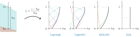
Vertical discretization schematic. The terrain-following coordinate ζ = (z − b_H)/h_H maps the ice column to [0,1]. Four vertical basis types are shown: Lagrange (piecewise polynomial interpolation), Legendre (polynomial expansion), MOLHO (Shallow Ice profile), and SSA (Shallow Shelf profile, depth-averaged).

Optimization set-up

With the velocity field discretized as DOF tensors \((\mathbf{u}_H, \mathbf{v}_H)\), the continuous energy minimization problem becomes a finite-dimensional optimization:

\[ \mathbf{u}_H^*, \mathbf{v}_H^* = \arg\min_{\mathbf{u}_H, \mathbf{v}_H} \mathcal{J}\left(\mathbf{u}_H, \mathbf{v}_H; \mathbf{c}_H, \mathbf{A}_H, \mathbf{h}_H, \mathbf{s}_H\right). \]

IGM supports two main computational strategies for solving this optimization problem, both minimizing the same physical energy functional \(\mathcal{J}\) but differing in what is optimized:

Direct velocity optimization (traditional solver): Optimize velocity degrees-of-freedom \((\mathbf{u}_H, \mathbf{v}_H)\) directly.
Neural network emulation (neural-network emulator): Optimize network weights that map the inputs \(\left(\mathbf{c}_H, \mathbf{A}_H, \mathbf{h}_H, \mathbf{s}_H\right)\) to the velocity degrees-of-freedom \((\mathbf{u}_H, \mathbf{v}_H)\).

The unified framework generalizes both strategies by introducing an abstract parameter vector \(\boldsymbol{\theta}\) and a mapping function \(\mathcal{M}\) that relates potential parameters to velocities:

\[ \boldsymbol{\theta}^* = \arg\min_{\boldsymbol{\theta}} \mathcal{J}\left(\mathcal{M}(\boldsymbol{\theta}); \mathbf{c}_H, \mathbf{A}_H, \mathbf{h}_H, \mathbf{s}_H\right), \quad (\mathbf{u}_H, \mathbf{v}_H) = \mathcal{M}(\boldsymbol{\theta}). \]

Mappings

Identity mapping: `unified.mapping: identity`

\[ \mathcal{M} = \mathcal{I} \quad \Rightarrow \quad (\mathbf{u}_H, \mathbf{v}_H) = \boldsymbol{\theta} \]

The parameters \(\boldsymbol{\theta}\) are the velocity degress-of-freedom themselves; the mapping is simply the identity mapping \(\mathcal{I}\). At each time step, the energy functional \(\mathcal{J}\) is minimized by optimizing \((\mathbf{u}_H, \mathbf{v}_H)\) directly given the current glacier state \((\mathbf{c}_H, \mathbf{A}_H, \mathbf{h}_H, \mathbf{s}_H)\). This is the traditional solver approach.

Network mapping: `unified.mapping: network`

\[ \mathcal{M} = \mathcal{N} \quad \Rightarrow \quad (\mathbf{u}_H, \mathbf{v}_H) = \mathcal{N}(\boldsymbol{\theta}) \]

The parameters \(\boldsymbol{\theta}\) are the weights of a neural network \(\mathcal{N}\) that maps glacier state \((\mathbf{c}_H, \mathbf{A}_H, \mathbf{h}_H, \mathbf{s}_H)\) to velocity degrees-of-freedom. Typically, the network can be a convolutional neural network (LeCun et al., 2015)⁹. Pretrained network can be chosen by specifying unified.network.pretrained: true.

Network mapping architecture

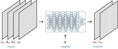
Network mapping architecture. The neural network parameterized by weights θ maps the glacier state (inputs: c_H, A_H, h_H, s_H) to velocity degrees of freedom (outputs: u_H, v_H).

Optimization algorithms

All optimizers operate on the abstract parameter \(\boldsymbol{\theta}\) via an iterative scheme:

\[ \boldsymbol{\theta}^{(k+1)} = \boldsymbol{\theta}^{(k)} + \alpha^{(k)} \, \mathbf{d}^{(k)}, \]

where \(\mathbf{d}^{(k)}\) is the search direction and \(\alpha^{(k)}\) is the step size. Typically, \(\mathbf{d}^{(k)}\) is computed based on the gradient \(\nabla_{\boldsymbol{\theta}} \mathcal{J}(\boldsymbol{\theta}^{(k)})\), which is computed automatically using TensorFlow's automatic differentiation.

Available optimizers:

Optimizer	Description	Reference
`adam`	Adaptive Moment Estimation: maintains running averages of gradient (first moment) and gradient magnitude (second moment)	(Kingma & Ba, 2015)¹⁰
`lbfgs`	Limited-memory BFGS: quasi-Newton method approximating the inverse Hessian using gradient history	(Nocedal & Wright, 2006)¹¹
`soap`	SOAP (Shampoo with Adam): second-order optimizer combining Shampoo-style preconditioned updates with Adam's moment estimation; effective for physics-informed neural network training	(Vyas et al., 2024)¹²
`sequential`	Multi-stage optimization allowing different optimizers and iteration counts in successive phases (see the quick start-up guide)	-

Convergence criteria

Optimization terminates when a success or failure criterion is met. Multiple criteria can be specified. Example configuration file:

unified:
  halt:
    success:
      - criterion: rel_tol
        metric: grad_u_norm
        tol: 1.0e-6
        ord: l2
    failure:
      - criterion: nan
      - criterion: inf

Success criteria: halt.success

Criterion	Description
`rel_tol`	Relative change in metric below tolerance
`abs_tol`	Absolute metric value below tolerance
`patience`	No improvement for specified iterations

Failure criteria: halt.failure

Criterion	Description
`nan`	NaN values detected
`inf`	Inf values detected

Metrics: metric

Metric	Description
`cost`	Energy functional value
`grad_u_norm`	Velocity gradient norm
`grad_theta_norm`	Parameter gradient norm
`u`	Velocity degrees-of-freedom
`theta`	Optimization parameters

Boundary conditions

Boundary conditions are configured via unified.bcs:

Condition	Equation
`frozen_bed`	\(\mathbf{u}\vert_{z=b} = \mathbf{0}\)
`periodic_ns`	\(\mathbf{u}\vert_{y=L_y} = \mathbf{u}\vert_{y=0}\)
`periodic_we`	\(\mathbf{u}\vert_{x=L_x} = \mathbf{u}\vert_{x=0}\)

Practical guidance

Choosing a mapping

Use identity for verification purposes — small domains and short simulations where you want to check that the solver is behaving correctly. Use network for production runs: it is faster and scales better to larger domains and longer projections.

Learning rates differ significantly between mappings

Always set both lr and lr_init explicitly — relying on defaults when switching mappings is a common source of problems.

mapping: identity — use lr / lr_init ≈ 0.9
mapping: network — use lr / lr_init in the range 1e-5 – 1e-3

A learning rate that is too high can cause numerical instabilities or a fully diverging run. If you observe velocities blowing up or NaN values in the output, reducing the learning rate is the first thing to try.

Validating `nbit`

nbit controls how many optimisation iterations are used per iceflow solve. Increasing it improves accuracy at the cost of compute time. A practical check: double nbit and verify that the resulting velocities change by less than ~5%.

To monitor convergence, watch the iceflow cost function value printed during the run — it should decrease and plateau. If it keeps oscillating or fails to decrease, try:

Increasing nbit.
Reducing the learning rate (lr / lr_init).
Running a short test with mapping: identity for comparison (remember to adjust lr / lr_init to ~0.9 for that case).

Checkerboard artefacts

When using the direct solver (mapping: identity), the default single-point cell-centred horizontal quadrature can admit checkerboard zero-energy modes — spurious oscillations in the velocity field where neighbouring cells move in opposite directions without contributing to the energy.

If you observe a checkerboard pattern in the velocity output, switch to a higher-order horizontal integration scheme via numerics.basis_horizontal:

Value	Scheme	Cost
`central`	Single cell-centred evaluation point (default)	Lowest, but susceptible to checkerboard modes
`q1`	2×2 Gaussian quadrature on bilinear (Q1) elements	Eliminates checkerboard modes
`p1`	P1 triangulation (each cell split into two triangles)	Eliminates checkerboard modes
`mac`	Marker-and-cell staggered-grid scheme	Eliminates checkerboard modes

Example configuration:

processes:
  iceflow:
    method: unified
    unified:
      mapping: identity
      numerics:
        basis_horizontal: q1   # or p1

Note

This issue is specific to the direct solver (mapping: identity). The neural-network emulator (mapping: network) is not affected because the network weights parameterize the velocity field globally, which inherently suppresses such spurious modes.

Choosing a vertical basis

Start with MOLHO (basis_vertical: molho, Nz: 2) — it captures the essential shear-sliding partition at low computational cost and is the recommended choice for most applications.

Switch to Lagrange with Nz between 4 and 10 only when a more detailed vertical velocity profile is needed (e.g. studies of englacial flow or vertical strain).

Common issues

Ice accumulating at domain borders

If ice builds up artificially along the edge of the domain, set exclude_borders_from_iceflow: True:

processes:
  iceflow:
    exclude_borders_from_iceflow: True

This prevents the solver from computing velocities in cells that touch the domain boundary, which can otherwise cause spurious accumulation.

Vertical velocity

The iceflow module can optionally compute the 3D vertical velocity field \(w\) (and its basal and surface projections \(w_\mathrm{b}\), \(w_\mathrm{s}\)) immediately after the horizontal velocity update. This sub-computation is disabled by default and enabled via:

iceflow:
  vertical_velocity:
    enabled: true   # default: false
    version: 2      # default: 2
    method: kinematic  # default: kinematic

When enabled, the following state variables are produced:

state.W — 3D vertical velocity field (shape Nz × Ny × Nx)
state.wvelbase — vertical velocity at the bed
state.wvelsurf — vertical velocity at the surface

Required for particles and enthalpy

Set iceflow.vertical_velocity.enabled: true when using 3D particle tracking (particles.tracking.method: "3d") or the enthalpy module for physically accurate vertical advection.

Physical principle

Both methods enforce the kinematic basal condition — that ice velocity is parallel to the bed:

\[ w_\mathrm{b} = u_\mathrm{b} \frac{\partial b}{\partial x} + v_\mathrm{b} \frac{\partial b}{\partial y}. \]

They differ in how \(w\) is extended through the column.

Kinematic method (`method: kinematic`)

The kinematic method requires that ice velocity be tangent to each terrain-following layer surface. At layer elevation \(z_\zeta = b + \zeta H\):

\[ w = u \frac{\partial z_\zeta}{\partial x} + v \frac{\partial z_\zeta}{\partial y} - \nabla \cdot (\bar{\mathbf{u}}_\zeta \, z_\zeta), \]

where \(\bar{\mathbf{u}}_\zeta\) is the depth-averaged velocity from the bed up to that layer. This naturally accounts for terrain through the layer-slope terms.

Incompressibility method (`method: incompressibility`)

The incompressibility method integrates the divergence-free condition \(\nabla \cdot \mathbf{u} = 0\) from the bed upward:

\[ w(\zeta) = w_\mathrm{b} - \int_0^\zeta \left(\frac{\partial u}{\partial x} + \frac{\partial v}{\partial y}\right) H\,\mathrm{d}\zeta'. \]

Because \(u\) and \(v\) are discretized at constant \(\zeta\) while the incompressibility condition requires horizontal derivatives at constant physical height \(z\), the derivatives must be transformed via the chain rule:

\[ \left.\frac{\partial u}{\partial x}\right|_z = \left.\frac{\partial u}{\partial x}\right|_\zeta - \left[\frac{\partial b}{\partial x} + \zeta\frac{\partial H}{\partial x}\right] \frac{\partial u}{\partial z}. \]

Versions

`version`	Kinematic	Incompressibility	Terrain correction	Implementation	Author
`1`	✓	✓	Kinematic only	Direct numerical derivatives	GJ
`2`	✓	✓	✓	Numerical integration with terrain chain rule	CMS
`3`	—	✓	✓	Matrix-based with precomputed operators	TG

Versions 1 and 2 support kinematic and incompressibility when using the Lagrange vertical basis. For Legendre basis, both use a spectral incompressibility method. For MOLHO basis, both use a two-layer kinematic approach. Version 3 implements only the incompressibility method for all bases.

Parameters

The complete default configuration file can be found here: iceflow.yaml.

Structure of the parameters:

iceflow
├── method
├── force_max_velbar
├── physics
│   └── ...
├── numerics
│   └── ...
├── solver
│   └── ...
├── emulator
│   └── ...
├── diagnostic
│   └── ...
├── unified
│   └── ...
└── vertical_velocity
    └── ...

Description of the parameters:

Name	Description	Default value	Units
`method`	Type of method to determine the ice flow: emulated, solved, diagnostic, unified.	unified	—
`force_max_velbar`	Upper-bound value for the velocities; applied if strictly positive.	0.0	m y\( ^{-1} \)

physics

Name	Description	Default value	Units
`physics.energy_components`	List of energy components to compute; the available components are: gravity, viscosity, sliding.	['viscosity', 'gravity', 'sliding']	—
`physics.sliding.law`	Type of sliding law.	weertman	—
`physics.sliding.use_mask_gr`	If True, zero out basal shear stress in floating areas.	False	—
`physics.sliding.slidingco`	Initial value for the reference basal shear stress (legacy stack: emulated/solved/diagnostic + data_assimilation; the field is named state.slidingco). Numerically equal to sliding.tau_ref.	0.0464	MPa
`physics.sliding.tau_ref`	Initial value for the reference basal shear stress (new stack: iceflow.method=unified + field_inversion + pretraining; the field is named state.tau_ref). Numerically equal to sliding.slidingco.	0.2153697218796329	MPa
`physics.sliding.regularization`	Regularization parameter for velocity magnitude (all laws).	1e-10	m y\( ^{-1} \)
`physics.sliding.exponent`	Sliding-law velocity exponent m (sliding stress ~ \|u\|^{1/m}). Applies to all laws.	3.0	—
`physics.sliding.u_ref`	Reference basal velocity. Active in the 'unified' method only (default 100 m/yr). The emulated/solved/diagnostic stack uses slidingco directly as tau_ref at u_ref=1 and refuses to run unless u_ref=1.0.	100.0	m y\( ^{-1} \)
`physics.sliding.N_ref`	Reference effective pressure (budd only; MPa, matching state.effective_pressure).	1.0	MPa
`physics.sliding.mu`	Till coefficient (regu_coulomb only).	0.4	—
`physics.sliding.q_exponent`	Effective-pressure exponent q (budd only). 1.0 recovers linear Budd, 0.5 gives Tsai sublinear.	1.0	—
`physics.sliding.phi`	Uniform friction angle (mohr_coulomb only). Used unless both bed_min and bed_max are finite.	30.0	deg
`physics.sliding.phi_min`	Friction angle at bed = bed_min (mohr_coulomb only).	15.0	deg
`physics.sliding.phi_max`	Friction angle at bed = bed_max (mohr_coulomb only).	45.0	deg
`physics.sliding.bed_min`	Lower bed elevation for friction-angle interpolation (mohr_coulomb only); NaN disables interpolation.	nan	m
`physics.sliding.bed_max`	Upper bed elevation for friction-angle interpolation (mohr_coulomb only); NaN disables interpolation.	nan	m
`physics.sliding.tauc_min`	Floor on tau_c after clipping (mohr_coulomb only).	0.1	MPa
`physics.sliding.tauc_max`	Ceiling on tau_c after clipping (mohr_coulomb only).	10000.0	MPa
`physics.sliding.tauc_ice_free`	Hard tau_c assignment in ice-free cells (mohr_coulomb only).	1.0	MPa
`physics.gravity_cst`	Gravitational constant.	9.81	m s\( ^{-2} \)
`physics.ice_density`	Density of ice.	910.0	kg m\( ^{-3} \)
`physics.water_density`	Density of water.	1000.0	kg m\( ^{-3} \)
`physics.viscosity.arrhenius`	Initial value for the Arrhenius factor in Glen's flow law.	78.0	MPa\( ^{-n} \) y\( ^{-1} \)
`physics.viscosity.enhancement_factor`	Enhancement factor in Glen's flow law: prefactor multiplying the arrhenius factor.	1.0	—
`physics.viscosity.exponent`	Glen's flow law exponent.	3.0	—
`physics.viscosity.regularization`	Regularization parameter for Glen's flow law.	1e-05	—
`physics.thr_ice_thk`	Minimal value for the ice thickness in the strain-rate computation.	0.1	m
`physics.min_sr`	Minimal value for the strain rate.	1e-20	y\( ^{-1} \)
`physics.max_sr`	Maximum value for the strain rate.	1e+20	y\( ^{-1} \)
`physics.force_negative_gravitational_energy`	Force the gravitational energy term to be negative.	False	—
`physics.cf_eswn`	This forces calving front at the border of the domain in the side given in the list.	[]	—

numerics

Name	Description	Default value	Units
`numerics.precision`	Precision type for the fields: single, double.	single	—
`numerics.ord_grad_u`	Default type of norm used for the halt critera associated with the velocity.	l2_weighted	—
`numerics.ord_grad_theta`	Default type of norm used for the halt critera associated with the parameters.	l2_weighted	—
`numerics.Nz`	Number of grid points for the vertical discretization.	4	—
`numerics.vert_spacing`	Parameter controlling the discretization density to get more points near the bed than near the surface; a value 1.0 means uniform vertical spacing.	4.0	—
`numerics.basis_horizontal`	Basis for the horizontal discretization.	central	—
`numerics.basis_vertical`	Basis for the vertical discretization.	Lagrange	—

solver

Name	Description	Default value	Units
`solver.step_size`	Step size for the optimizer.	1.0	—
`solver.nbitmax`	Maximum number of iterations for the optimizer.	100	—
`solver.optimizer`	Type of optimizer.	adam	—
`solver.print_cost`	Display the cost during the optimization.	False	—
`solver.fieldin`	Input fields of the ice-flow solver.	['thk', 'usurf', 'arrhenius', 'slidingco', 'dX']	—

emulator

Name	Description	Default value	Units
`emulator.fieldin`	Input fields of the ice-flow emulator.	['thk', 'usurf', 'arrhenius', 'slidingco', 'dX']	—
`emulator.retrain_freq`	Frequency at which the emulator is retrained.	10	—
`emulator.print_cost`	Display the cost during the optimization.	False	—
`emulator.lr`	Learning rate for the training of the emulator.	2e-05	—
`emulator.lr_init`	Initial learning rate for the training of the emulator.	0.0001	—
`emulator.lr_decay`	Decay learning-rate parameter for the training of the emulator.	0.95	—
`emulator.warm_up_it`	Number of iterations for a warm-up period, allowing intense initial training.	-10000000000.0	—
`emulator.nbit_init`	Number of iterations done initially for the training of the emulator.	1	—
`emulator.nbit`	Number of iterations done at each time step for the training of the emulator.	1	—
`emulator.framesizemax`	Size of the patch used for training the emulator; this is useful for large size arrays as otherwise the GPU memory could be overloaded.	1000	—
`emulator.split_patch_method`	Method to split the patch for the emulator: sequential (usefull for large size arrays) or parallel.	sequential	—
`emulator.pretrained`	Use a pretrained emulator instead of starting from scratch.	True	—
`emulator.name`	Directory path of the pretrained ice-flow emulator; taken from the library if this is empty.		—
`emulator.save_model`	Save the ice-flow emulator at the end of the simulation.	False	—
`emulator.exclude_borders`	Quick fix of the border issue; otherwise the emulator shows zero velocity at the border.	0	—
`emulator.optimizer`	Type of optimizer for the emulator.	Adam	—
`emulator.optimizer_clipnorm`	Maximum value for the gradient of each weight.	1.0	—
`emulator.optimizer_epsilon`	Small constant for numerical stability of the Adam optimizer.	1e-07	—
`emulator.save_cost`	Name of the file containing the cost.		—
`emulator.output_directory`	Directory of the file containing the cost.		—
`emulator.plot_sol`	Plot the solution of the emulator at each time step.	False	—
`emulator.pertubate`	Perturb the input fiels during the training.	False	—
`emulator.network.architecture`	Type of network: cnn, unet.	cnn	—
`emulator.network.params`		{}
`emulator.network.multiple_window_size`	For a U-Net, this requires the window size to be a multiple of 2 to the power N.	0	—
`emulator.network.activation`	Type of activation function: lrelu, relu, tanh, sigmoid, ...	LeakyReLU	—
`emulator.network.nb_layers`	Number of layers in the network.	16	—
`emulator.network.nb_blocks`	Number of block layers in the U-Net.	4	—
`emulator.network.nb_out_filter`	Number of output filters in the network.	32	—
`emulator.network.conv_ker_size`	Size of the convolution kernel.	3	—
`emulator.network.dropout_rate`	Dropout rate in the CNN.	0.0	—
`emulator.network.weight_initialization`	Initialization type for the network weights: glorot_uniform, he_normal, lecun_normal.	glorot_uniform	—
`emulator.network.cnn3d_for_vertical`	Apply a 3D CNN instead of a 2D one for each horizontal layer.	False	—
`emulator.network.batch_norm`	Apply a batch normalization layer.	False	—
`emulator.network.l2_reg`	Amount of l2 regularization penalty.	0.0	—
`emulator.network.separable`	Apply convolution layers that are separable.	False	—
`emulator.network.residual`	Apply residual layer.	True	—

diagnostic

Name	Description	Default value	Units
`diagnostic.save_freq`	Frequency of the saving of the metrics.	1	—
`diagnostic.filename_metrics`	Name of the file with the metrics.	diagnostic_metrics.txt	—

unified

Name	Description	Default value	Units
`unified.mapping`	Type of mapping between the weights and the velocity.	network	—
`unified.bcs`	List of the applied boundary conditions; the available bcs are: frozen_bed, periodic_ns, periodic_we, no_slip, periodic_ns_global, periodic_we_global, no_slip_global.	[]	—
`unified.bc.dirichlet.left`	Value enforced on the DOFs of the velocity at the left (west) border; note that this sets the degrees of freedom, not the velocity field itself.	0.0	m y\( ^{-1} \)
`unified.bc.dirichlet.right`	Value enforced on the DOFs of the velocity at the right (east) border; note that this sets the degrees of freedom, not the velocity field itself.	0.0	m y\( ^{-1} \)
`unified.bc.dirichlet.top`	Value enforced on the DOFs of the velocity at the top (north) border; note that this sets the degrees of freedom, not the velocity field itself.	0.0	m y\( ^{-1} \)
`unified.bc.dirichlet.bottom`	Value enforced on the DOFs of the velocity at the bottom (south) border; note that this sets the degrees of freedom, not the velocity field itself.	0.0	m y\( ^{-1} \)
`unified.optimizer`	Type of optimizer used to solve the ice flow.	adam	—
`unified.nbit`	Number of iterations done to solve the ice flow.	5	—
`unified.nbit_init`	Number of iterations done initially to solve the ice flow.	300	—
`unified.nbit_warmup`	Number of iterations done for a warm-up period to solve the ice flow, allowing intense initial training.	-1	—
`unified.retrain_freq`	Frequency at which the ice flow is solved.	5	—
`unified.retrain_threshold`	Threshold (expressed as a z-score) above which the ice flow is re-solved.	10000000000.0	—
`unified.newton.damping`		1e-6
`unified.adam.lr`	Learning rate for the Adam optimizer.	0.0005	—
`unified.adam.lr_init`	Initial learning rate for the Adam optimizer.	0.002	—
`unified.adam.lr_decay`	Decay learning-rate parameter for the Adam optimizer.	1.0	—
`unified.adam.lr_decay_steps`	Number of steps during which the decay learning rate is applied for the Adam optimizer.	1000	—
`unified.adam.optimizer_clipnorm`	Maximum value for the gradient of each weight.	1.0	—
`unified.lbfgs.memory`	Number of saved iteration results for the L-BFGS optimizer.	10	—
`unified.lbfgs.alpha_min`	Minimal value for the step size in the line search.	0.0	—
`unified.cg_newton.cg_tol`	Tolerance for the conjugate-gradient linear solver in the CG-Newton optimizer.	1e-10	—
`unified.cg_newton.cg_max_iter`	Maximum number of conjugate-gradient iterations in the CG-Newton optimizer.	100	—
`unified.cg_newton.truncated`	Use truncated (inexact) Newton steps in the CG-Newton optimizer.	True	—
`unified.cg_newton.damping`	Damping added to the Hessian diagonal for regularization in the CG-Newton optimizer.	1e-6	—
`unified.trust_region.cg_max_iter`	Maximum number of conjugate-gradient iterations for the trust-region sub-problem.	100	—
`unified.trust_region.cg_tol`	Tolerance for the conjugate-gradient linear solver in the trust-region optimizer.	1e-12	—
`unified.trust_region.delta_init`	Initial trust-region radius.	1e2	—
`unified.trust_region.delta_max`	Maximum trust-region radius.	1e10	—
`unified.trust_region.eta`	Minimum ratio of actual to predicted reduction for accepting a step in the trust-region optimizer.	0.15	—
`unified.trust_region.damping`	Damping added to the Hessian diagonal for regularization in the trust-region optimizer.	1e-6	—
`unified.muon.lr`	Learning rate for matrix parameters (conv kernels, Dense kernels) in the Muon optimizer.	0.02	—
`unified.muon.momentum`	Nesterov momentum coefficient for the Muon optimizer.	0.95	—
`unified.muon.ns_steps`	Number of Newton-Schulz iterations used to orthogonalize the gradient update in the Muon optimizer.	5	—
`unified.muon.lr_1d`	Learning rate for rank-1 parameters (biases) in the Muon optimizer; these receive plain Nesterov SGD.	0.0003	—
`unified.soap.lr`	Adam learning rate for the SOAP optimizer.	0.0003	—
`unified.soap.beta1`	Adam first-moment decay coefficient for the SOAP optimizer.	0.95	—
`unified.soap.beta2`	Adam second-moment decay coefficient for the SOAP optimizer; also used to update the Kronecker preconditioner factors.	0.999	—
`unified.soap.eps`	Epsilon for numerical stability in the Adam update of the SOAP optimizer.	1e-08	—
`unified.soap.precond_freq`	Number of iterations between eigendecompositions of the Kronecker preconditioner factors in the SOAP optimizer.	10	—
`unified.soap.damping`	Regularization added to the Kronecker preconditioner factors before eigendecomposition in the SOAP optimizer.	1e-08	—
`unified.sequential.stages`	List containing the optimizer configurations when using a sequential optimization approach.	[]	—
`unified.line_search`	Type of line-search method.	hager-zhang	—
`unified.inputs`	Input fields of the mapping for the ice flow.	['thk', 'usurf', 'arrhenius', 'tau_ref', 'dX']	—
`unified.normalization.method`	Type of method used for the normalization of the inputs: adaptive, fixed.	adaptive	—
`unified.normalization.fixed.inputs_offsets.thk`	Fixed offset for the input thk.	0.0	m
`unified.normalization.fixed.inputs_offsets.usurf`	Fixed offset for the input usurf.	0.0	m
`unified.normalization.fixed.inputs_offsets.arrhenius`	Fixed offset for the input arrhenius.	0.0	MPa\( ^{-n} \) y\( ^{-1} \)
`unified.normalization.fixed.inputs_offsets.tau_ref`		0.0
`unified.normalization.fixed.inputs_offsets.dX`	Fixed offset for the input dX.	0.0	m
`unified.normalization.fixed.inputs_offsets.X`	Fixed offset for the input X.	0.0	m
`unified.normalization.fixed.inputs_offsets.Y`	Fixed offset for the input Y.	0.0	m
`unified.normalization.fixed.inputs_variances.thk`	Fixed variance for the input thk.	1.0	m
`unified.normalization.fixed.inputs_variances.usurf`	Fixed variance for the input usurf.	1.0	m
`unified.normalization.fixed.inputs_variances.arrhenius`	Fixed variance for the input arrhenius.	1.0	MPa\( ^{-n} \) y\( ^{-1} \)
`unified.normalization.fixed.inputs_variances.tau_ref`		1.0
`unified.normalization.fixed.inputs_variances.dX`	Fixed variance for the input dX.	1.0	m
`unified.normalization.fixed.inputs_variances.X`	Fixed variance for the input X.	1.0	m
`unified.normalization.fixed.inputs_variances.Y`	Fixed variance for the input Y.	1.0	m
`unified.network.debug_mode`	Enable debug mode for the optimizer.	False	—
`unified.network.debug_freq`	Frequency of debug output.	100	—
`unified.network.pretrained`	Use a pretrained network instead of starting from scratch.	False	—
`unified.network.pretrained_path`	Path to the pretrained network; taken from the library if empty.		—
`unified.network.print_summary`	Print a summary of the network.	False	—
`unified.network.output_scale`	Scale of the outputs of the network.	1.0	—
`unified.network.architecture`	Type of network.	dahunet	—
`unified.network.params`	Architecture hyperparameters for the from-scratch path (pretrained: false), owned by the unified mode (no longer read from emulator.network). Keys depend on `architecture`; an empty dict uses the architecture's built-in defaults.	{'backend': 'cnn', 'features': ['dsdx', 'dsdy', 'grad_s', 'u_sia', 'u_weertman'], 'nb_out_filter': 24, 'nb_layers': 6, 'conv_ker_size': 3, 'residual': True}	—
`unified.data_preparation.framesizemax`	Maximum patch size; the domain is split into non-overlapping patches no larger than this value to avoid GPU memory overload.	99999	—
`unified.data_preparation.patches_per_batch`	Number of patches processed per mini-batch during optimization.	1	—
`unified.halt.freq`	Frequency of evaluation of the halt criteria.	1	—
`unified.halt.success`	List of success criteria.	[]	—
`unified.halt.failure`	List of failure criteria.	[]	—
`unified.halt.criteria.rel_tol.tol`	Default tolerance for the relative-change criterion.	1e-3	—
`unified.halt.criteria.rel_tol.ord`	Default type of norm for the relative-change criterion.	l2	—
`unified.halt.criteria.abs_tol.tol`	Default tolerance for the absolute-change criterion.	1e-3	—
`unified.halt.criteria.abs_tol.ord`	Default type of norm for the absolute-change criterion.	l2_weighted	—
`unified.halt.criteria.patience.patience`	Default number of iteration without improvement before halting.	100	—
`unified.halt.criteria.inf`	Default parameters for the inf criterion.	{}	—
`unified.halt.criteria.nan`	Default parameters for the nan criterion.	{}	—
`unified.halt.metrics.theta`	Default parameters for the parameter metric.	{}	—
`unified.halt.metrics.u`	Default parameters for the velocity metric.	{}	—
`unified.halt.metrics.cost`	Default parameters for the cost metric.	{}	—
`unified.halt.metrics.grad_u_norm`	Default parameters for the velocity-gradient-of-the-cost metric.	{}	—
`unified.halt.metrics.grad_theta_norm`	Default parameters for the parameter-gradient-of-the-cost metric.	{}	—
`unified.display.print_cost`	Print the cost during the ice-flow optimization.	False	—
`unified.display.print_cost_freq`	Frequency of printing the cost during the ice-flow optimization.	1	—

vertical_velocity

Name	Description	Default value	Units
`vertical_velocity.enabled`	Activate vertical velocity computation (W, wvelbase, wvelsurf) after the iceflow update. Required for 3D particle tracking and enthalpy vertical advection.	False	—
`vertical_velocity.version`	Version of the vertical_velocity method (1: original by GJ; 2: improved by CMS; 3: unified by TG).	2	—
`vertical_velocity.method`	Method to retrieve the vertical velocity: kinematic (layer-following) or incompressibility (divergence-free). Version 3 only supports incompressibility.	kinematic	—

Contributors: Guillaume Jouvet, Thomas Gregov, Brandon Finley, Sebastian Rosier, Claire-Mathile Stücki.

The IGM developers. (in prep.). IGM: An accessible, modular, differentiable, and GPU-accelerated high-order ice flow model. https://doi.org/10.31223/X5GB6G ↩
Herterich, K. (1987). On the flow within the transition zone between ice sheet and ice shelf. In Dynamics of the west antarctic ice sheet (pp. 185--202). Springer Netherlands. https://doi.org/10.1007/978-94-009-3745-1\_11 ↩
Blatter, H. (1995). Velocity and stress fields in grounded glaciers: A simple algorithm for including deviatoric stress gradients. Journal of Glaciology, 41(138), 333--344. https://doi.org/10.3189/s002214300001621x ↩
Pattyn, F. (2003). A new three‐dimensional higher‐order thermomechanical ice sheet model: Basic sensitivity, ice stream development, and ice flow across subglacial lakes. Journal of Geophysical Research: Solid Earth, 108(B8). https://doi.org/10.1029/2002jb002329 ↩
Jouvet, G., & Rappaz, J. (2011). Analysis and finite element approximation of a nonlinear stationary stokes problem arising in glaciology. Advances in Numerical Analysis, 2011, 1--24. https://doi.org/10.1155/2011/164581 ↩
Jouvet, G. (2016). Mechanical error estimators for shallow ice flow models. Journal of Fluid Mechanics, 807, 40--61. https://doi.org/10.1017/jfm.2016.593 ↩
Jouvet, G., & Cordonnier, G. (2023). Ice-flow model emulator based on physics-informed deep learning. Journal of Glaciology, 1--15. https://doi.org/10.1017/jog.2023.73 ↩
Dias dos Santos, T., Morlighem, M., & Brinkerhoff, D. (2022). A new vertically integrated MOno-Layer Higher-Order (MOLHO) ice flow model. The Cryosphere, 16(1), 179--195. https://doi.org/10.5194/tc-16-179-2022 ↩
LeCun, Y., Bengio, Y., & Hinton, G. (2015). Deep learning. Nature, 521, 436--444. https://doi.org/10.1038/nature14539 ↩
Kingma, D. P., & Ba, J. (2015). Adam: A method for stochastic optimization. 3rd International Conference on Learning Representations, ICLR 2015. http://arxiv.org/abs/1412.6980 ↩
Nocedal, J., & Wright, S. J. (2006). Numerical optimization (2nd ed.). Springer New York. https://doi.org/10.1007/978-0-387-40065-5 ↩
Vyas, N., Morwani, D., Zhao, R., Kwun, I., Shapira, I., Brandfonbrener, D., Janson, L., & Kakade, S. (2024). SOAP: Improving and stabilizing Shampoo using Adam. https://doi.org/10.48550/arXiv.2409.11321 ↩

Module iceflow

Quick start-up guide

Legacy modes

Unified mode

Physical model

Minimization formulation

Numerical set-up

Horizontal discretization

Vertical discretization

Vertical basis functions

Optimization set-up

Mappings

Identity mapping: unified.mapping: identity

Network mapping: unified.mapping: network

Optimization algorithms

Convergence criteria

Boundary conditions

Practical guidance

Choosing a mapping

Validating nbit

Checkerboard artefacts

Choosing a vertical basis

Common issues

Vertical velocity

Physical principle

Kinematic method (method: kinematic)

Incompressibility method (method: incompressibility)

Versions

Parameters

Module `iceflow`

Identity mapping: `unified.mapping: identity`

Network mapping: `unified.mapping: network`

Validating `nbit`

Kinematic method (`method: kinematic`)

Incompressibility method (`method: incompressibility`)